How To Draw Corresponding V Vs T And A Vs T For Curved Position And Time Graphs

Until next time

This tutorial explains matplotlib's way of making plots in simplified parts so yous gain the cognition and a clear understanding of how to build and modify full featured matplotlib plots.

1. Introduction

Matplotlib is the nigh pop plotting library in python. Using matplotlib, you can create pretty much whatever type of plot. Yet, as your plots get more than complex, the learning curve tin can get steeper.

The goal of this tutorial is to make y'all sympathise 'how plotting with matplotlib works' and make you comfortable to build full-featured plots with matplotlib.

2. A Basic Scatterplot

The post-obit piece of lawmaking is found in pretty much any python code that has matplotlib plots.

          import matplotlib.pyplot as plt %matplotlib inline                  

matplotlib.pyplot is normally imported as plt. It is the core object that contains the methods to create all sorts of charts and features in a plot.

The %matplotlib inline is a jupyter notebook specific command that let's yous see the plots in the notbook itself.

Suppose you want to draw a specific type of plot, say a scatterplot, the first affair yous want to bank check out are the methods under plt (blazon plt and hitting tab or blazon dir(plt) in python prompt).

Let's begin by making a elementary but total-featured scatterplot and take it from there. Let's see what plt.plot() creates if you an arbitrary sequence of numbers.

          import matplotlib.pyplot as plt %matplotlib inline  # Plot plt.plot([1,2,three,4,10]) #> [<matplotlib.lines.Line2D at 0x10edbab70>]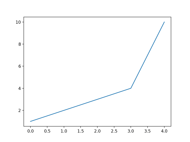                  

I just gave a listing of numbers to plt.plot() and it drew a line chart automatically. It assumed the values of the Ten-axis to start from nil going up to as many items in the data.

Find the line matplotlib.lines.Line2D in code output?

That'due south because Matplotlib returns the plot object itself besides drawing the plot.

If you only want to see the plot, add plt.show() at the cease and execute all the lines in one shot.

Alright, notice instead of the intended scatter plot, plt.plot drew a line plot. That'south because of the default behaviour.

So how to draw a scatterplot instead?

Well to practise that, allow'southward sympathise a bit more nearly what arguments plt.plot() expects. The plt.plot accepts 3 basic arguments in the following guild: (x, y, format).

This format is a brusque hand combination of {color}{marker}{line}.

For case, the format 'go-' has 3 characters continuing for: 'green colored dots with solid line'. By omitting the line role ('-') in the end, y'all will be left with just green dots ('go'), which makes it describe a scatterplot.

Few commonly used brusk hand format examples are:
* 'r*--' : 'carmine stars with dashed lines'
* 'ks.' : 'black squares with dotted line' ('thousand' stands for black)
* 'bD-.' : 'bluish diamonds with dash-dot line'.

For a complete list of colors, markers and linestyles, bank check out the aid(plt.plot) control.

Allow's draw a scatterplot with greendots.

          # 'go' stands for green dots plt.plot([1,two,iii,four,5], [one,2,three,iv,10], 'get') plt.bear witness()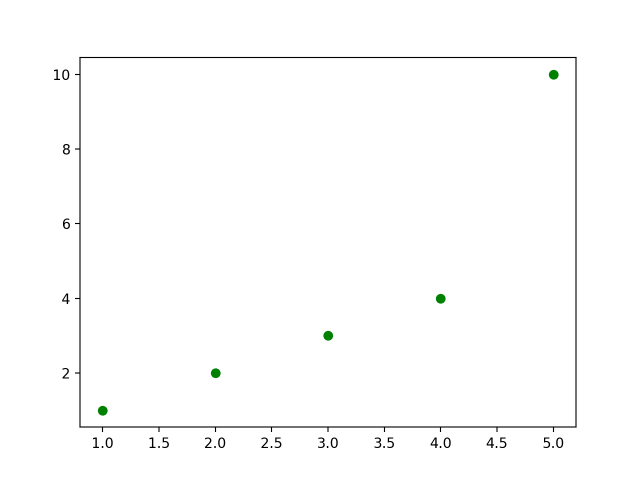                  

three. How to draw two sets of scatterplots in same plot

Skilful. Now how to plot another set of five points of different color in the same figure?

Only call plt.plot() again, it will add those point to the aforementioned film.

You might wonder, why it does not draw these points in a new panel birthday? I will come to that in the side by side section.

          # Draw two sets of points plt.plot([1,ii,3,4,5], [1,two,3,4,x], 'get')  # green dots plt.plot([i,2,three,iv,5], [ii,iii,4,5,eleven], 'b*')  # blueish stars plt.bear witness()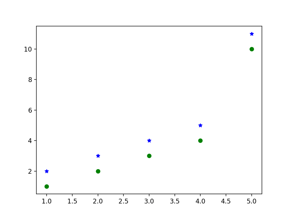                  

Looks good. Now permit's add the basic plot features: Title, Legend, X and Y axis labels. How to do that?

The plt object has respective methods to add together each of this.

          plt.plot([1,2,3,four,5], [i,2,3,4,10], 'go', characterization='GreenDots') plt.plot([1,2,3,4,5], [2,3,4,v,xi], 'b*', label='Bluestars') plt.championship('A Simple Scatterplot') plt.xlabel('X') plt.ylabel('Y') plt.legend(loc='best')  # legend text comes from the plot's label parameter. plt.show()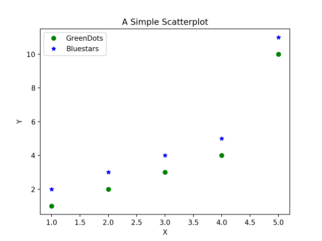                  

Good. At present, how to increase the size of the plot? (The higher up plot would actually look minor on a jupyter notebook)

The easy style to practise information technology is by setting the figsize inside plt.figure() method.

          plt.figure(figsize=(x,7)) # ten is width, vii is acme plt.plot([one,2,3,4,5], [ane,2,3,4,10], 'go', label='GreenDots')  # green dots plt.plot([1,2,3,4,5], [2,3,4,5,eleven], 'b*', label='Bluestars')  # bluish stars plt.championship('A Simple Scatterplot')   plt.xlabel('X') plt.ylabel('Y') plt.xlim(0, 6) plt.ylim(0, 12) plt.legend(loc='best') plt.show()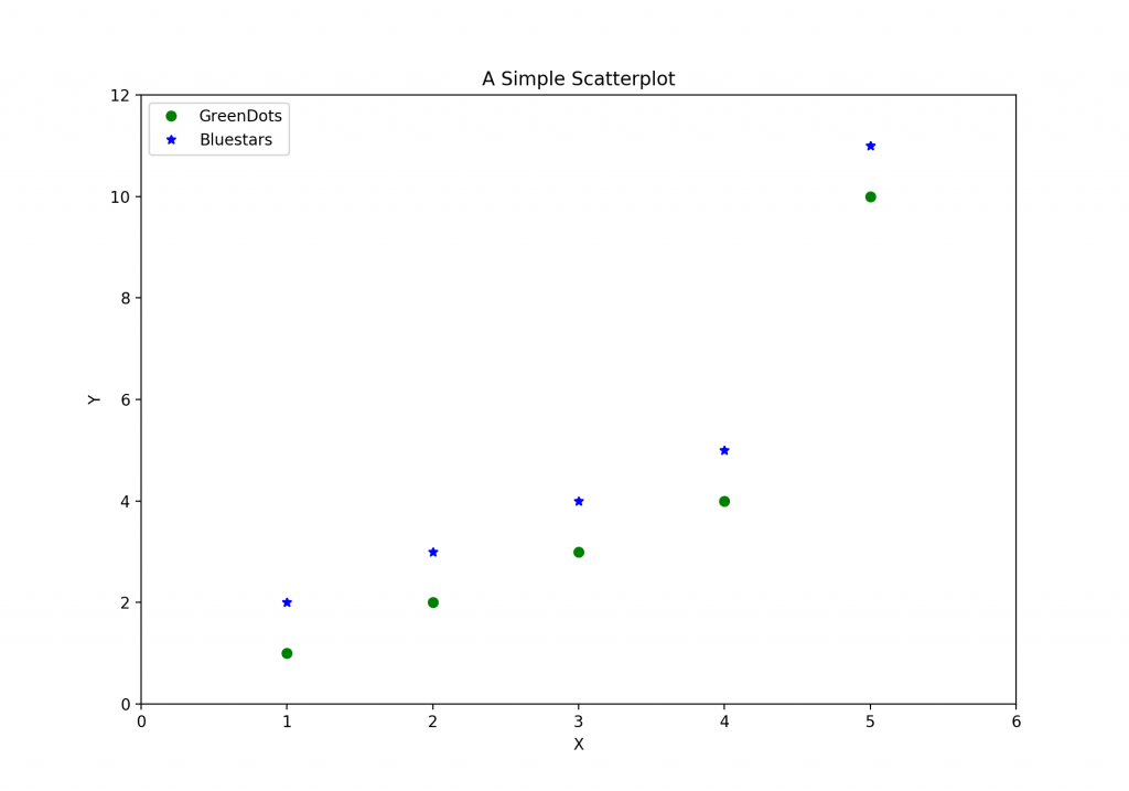                  

Ok, nosotros accept some new lines of code there. What does plt.figure do?

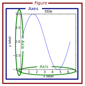
Well, every plot that matplotlib makes is fatigued on something chosen 'figure'. You lot can think of the figure object as a sheet that holds all the subplots and other plot elements inside it.

And a effigy tin can have one or more subplots inside information technology called axes, arranged in rows and columns. Every effigy has atleast one axes. (Don't misfile this axes with 10 and Y axis, they are different.)

4. How to draw two scatterplots in dissimilar panels

Permit's understand figure and axes in little more detail.

Suppose, I want to depict our ii sets of points (green rounds and blueish stars) in ii separate plots side-by-side instead of the aforementioned plot. How would you exercise that?

Yous tin can do that by creating ii separate subplots, aka, axes using plt.subplots(1, 2). This creates and returns ii objects:
* the effigy
* the axes (subplots) inside the figure

Previously, I called plt.plot() to describe the points. Since there was merely one axes by default, information technology drew the points on that axes itself.

But now, since you desire the points drawn on unlike subplots (axes), yous take to call the plot office in the respective axes (ax1 and ax2 in beneath code) instead of plt.

Notice in below code, I call ax1.plot() and ax2.plot() instead of calling plt.plot() twice.

          # Create Effigy and Subplots fig, (ax1, ax2) = plt.subplots(1,ii, figsize=(ten,4), sharey=True, dpi=120)  # Plot ax1.plot([one,2,3,4,5], [i,two,3,4,10], 'go')  # greendots ax2.plot([1,ii,three,4,5], [2,iii,iv,5,11], 'b*')  # bluestart  # Title, X and Y labels, X and Y Lim ax1.set_title('Scatterplot Greendots'); ax2.set_title('Scatterplot Bluestars') ax1.set_xlabel('10');  ax2.set_xlabel('X')  # 10 label ax1.set_ylabel('Y');  ax2.set_ylabel('Y')  # y label ax1.set_xlim(0, 6) ;  ax2.set_xlim(0, 6)   # x axis limits ax1.set_ylim(0, 12);  ax2.set_ylim(0, 12)  # y axis limits  # ax2.yaxis.set_ticks_position('none')  plt.tight_layout() plt.evidence()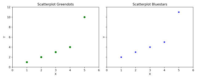                  

Setting sharey=True in plt.subplots() shares the Y axis between the two subplots.

And dpi=120 increased the number of dots per inch of the plot to make it await more sharp and clear. You volition find a singled-out improvement in clarity on increasing the dpi especially in jupyter notebooks.

Thats sounds like a lot of functions to learn. Well it's quite like shooting fish in a barrel to remember information technology really.

The ax1 and ax2 objects, like plt, has equivalent set_title, set_xlabel and set_ylabel functions. Infact, the plt.title() actually calls the current axes set_title() to do the job.

• plt.xlabel() ? ax.set_xlabel()
• plt.ylabel() ? ax.set_ylabel()
• plt.xlim() ? ax.set_xlim()
• plt.ylim() ? ax.set_ylim()
• plt.title() ? ax.set_title()

Alternately, to save keystrokes, yous can fix multiple things in one go using the ax.set().

          ax1.set(title='Scatterplot Greendots', xlabel='10', ylabel='Y', xlim=(0,6), ylim=(0,12)) ax2.set(title='Scatterplot Bluestars', xlabel='Ten', ylabel='Y', xlim=(0,6), ylim=(0,12))                  

5. Object Oriented Syntax vs Matlab like Syntax

A known 'problem' with learning matplotlib is, information technology has two coding interfaces:

1. Matlab like syntax
2. Object oriented syntax.

This is partly the reason why matplotlib doesn't accept one consistent style of achieving the aforementioned given output, making it a flake difficult to sympathise for new comers.

The syntax yous've seen so far is the Object-oriented syntax, which I personally prefer and is more intuitive and pythonic to work with.

However, since the original purpose of matplotlib was to recreate the plotting facilities of matlab in python, the matlab-like-syntax is retained and still works.

The matlab syntax is 'stateful'.

That means, the plt keeps rails of what the current axes is. So whatever you describe with plt.{anything} volition reflect only on the electric current subplot.

Practically speaking, the main deviation betwixt the 2 syntaxes is, in matlab-like syntax, all plotting is done using plt methods instead of the respective axes's method as in object oriented syntax.

So, how to recreate the to a higher place multi-subplots figure (or any other figure for that matter) using matlab-like syntax?

The general procedure is: You manually create one subplot at a time (using plt.subplot() or plt.add_subplot()) and immediately telephone call plt.plot() or plt.{anything} to modify that specific subplot (axes). Any method you phone call using plt will be fatigued in the current axes.

The lawmaking below shows this in practice.

          plt.effigy(figsize=(10,four), dpi=120) # 10 is width, 4 is height  # Left hand side plot plt.subplot(i,2,1)  # (nRows, nColumns, axes number to plot) plt.plot([1,ii,iii,4,five], [1,ii,3,four,x], 'go')  # green dots plt.title('Scatterplot Greendots')   plt.xlabel('X'); plt.ylabel('Y') plt.xlim(0, half-dozen); plt.ylim(0, 12)  # Correct hand side plot plt.subplot(1,two,two) plt.plot([one,2,3,4,5], [2,iii,4,5,11], 'b*')  # blueish stars plt.title('Scatterplot Bluestars')   plt.xlabel('X'); plt.ylabel('Y') plt.xlim(0, 6); plt.ylim(0, 12) plt.bear witness()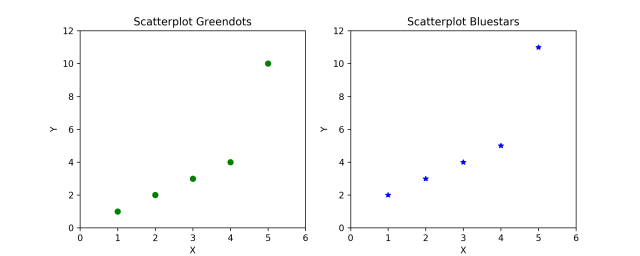                  

Let'south breakdown the above piece of code.

In plt.subplot(1,2,1), the kickoff ii values, that is (1,2) specifies the number of rows (1) and columns (2) and the third parameter (1) specifies the position of current subplot. The subsequent plt functions, volition always draw on this current subplot.

You can get a reference to the current (subplot) axes with plt.gca() and the current figure with plt.gcf(). Likewise, plt.cla() and plt.clf() will clear the current axes and figure respectively.

Alright, compare the in a higher place code with the object oriented (OO) version. The OO version might look a only confusing because it has a mix of both ax1 and plt commands.

Notwithstanding, at that place is a pregnant advantage with axes approach.

That is, since plt.subplots returns all the axes as split up objects, y'all can avoid writing repetitive lawmaking by looping through the axes.

Always remember: plt.plot() or plt.{anything} will always act on the plot in the current axes, whereas, ax.{annihilation} volition modify the plot inside that specific ax.

          # Describe multiple plots using for-loops using object oriented syntax import numpy as np from numpy.random import seed, randint seed(100)  # Create Figure and Subplots fig, axes = plt.subplots(2,2, figsize=(10,6), sharex=True, sharey=True, dpi=120)  # Ascertain the colors and markers to apply colors = {0:'g', ane:'b', 2:'r', 3:'y'} markers = {0:'o', 1:'x', 2:'*', 3:'p'}  # Plot each axes for i, ax in enumerate(axes.ravel()):     ax.plot(sorted(randint(0,10,x)), sorted(randint(0,10,x)), marker=markers[i], color=colors[i])       ax.set_title('Ax: ' + str(i))     ax.yaxis.set_ticks_position('none')  plt.suptitle('Four Subplots in One Figure', verticalalignment='bottom', fontsize=sixteen)     plt.tight_layout() plt.evidence()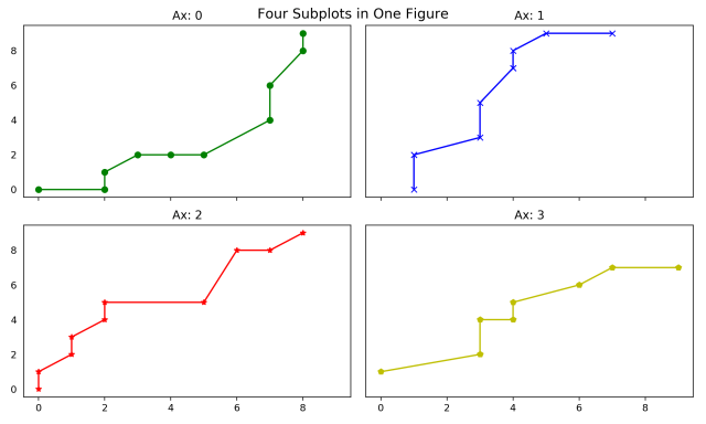                  

Did you notice in above plot, the Y-axis does not have ticks?

That'south because I used ax.yaxis.set_ticks_position('none') to turn off the Y-axis ticks. This is some other advantage of the object-oriented interface. Y'all can actually get a reference to any specific chemical element of the plot and utilize its methods to dispense it.

Can you guess how to turn off the 10-axis ticks?

The plt.suptitle() added a master championship at effigy level title. plt.championship() would have washed the same for the electric current subplot (axes).

The verticalalignment='bottom' parameter denotes the hingepoint should be at the bottom of the title text, then that the chief title is pushed slightly up.

Alright, What you've learned so far is the core essence of how to create a plot and manipulate it using matplotlib. Next, permit's see how to get the reference to and modify the other components of the plot

6. How to Modify the Centrality Ticks Positions and Labels

There are three basic things you will probably ever need in matplotlib when information technology comes to manipulating axis ticks:
i. How to command the position and tick labels? (using plt.xticks() or ax.set upxticks() and ax.setxticklabels())
ii. How to command which axis'south ticks (tiptop/bottom/left/correct) should be displayed (using plt.tick_params())
3. Functional formatting of tick labels

If you are using ax syntax, y'all can utilize ax.set_xticks() and ax.set_xticklabels() to set the positions and label texts respectively. If you are using the plt syntax, you can set both the positions also equally the label text in ane call using the plt.xticks().

Actually, if you look at the code of plt.xticks() method (past typing ??plt.xticks in jupyter notebook), it calls ax.set_xticks() and ax.set_xticklabels() to practise the job. plt.xticks takes the ticks and labels as required parameters but y'all can also accommodate the characterization'southward fontsize, rotation, 'horizontalalignment' and 'verticalalignment' of the hinge points on the labels, like I've washed in the below example.

          from matplotlib.ticker import FuncFormatter  def rad_to_degrees(10, pos):     'converts radians to degrees'     return circular(ten * 57.2985, two)  plt.figure(figsize=(12,7), dpi=100) X = np.linspace(0,2*np.pi,1000) plt.plot(10,np.sin(X)) plt.plot(X,np.cos(Ten))  # i. Accommodate ten axis Ticks plt.xticks(ticks=np.arange(0, 440/57.2985, 90/57.2985), fontsize=12, rotation=30, ha='center', va='superlative')  # i radian = 57.2985 degrees  # 2. Tick Parameters plt.tick_params(axis='both',bottom=True, height=True, left=True, right=True, direction='in', which='major', grid_color='blue')  # 3. Format tick labels to catechumen radians to degrees formatter = FuncFormatter(rad_to_degrees) plt.gca().xaxis.set_major_formatter(formatter)  plt.grid(linestyle='--', linewidth=0.5, alpha=0.fifteen) plt.title('Sine and Cosine Waves\northward(Observe the ticks are on all 4 sides pointing inwards, radians converted to degrees in ten axis)', fontsize=fourteen) plt.show()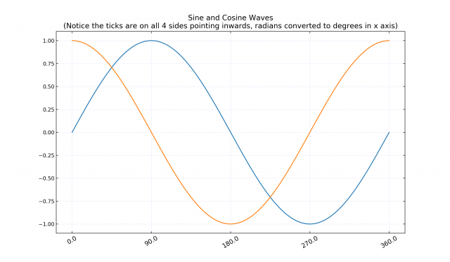                  

In to a higher place lawmaking, plt.tick_params() is used to make up one's mind which all centrality of the plot ('top' / 'bottom' / 'left' / 'right') y'all desire to draw the ticks and which direction ('in' / 'out') the tick should point to.

the matplotlib.ticker module provides the FuncFormatter to determine how the final tick label should be shown.

7. Agreement the rcParams, Colors and Plot Styles

The look and feel of various components of a matplotlib plot tin be gear up globally using rcParams. The complete list of rcParams can be viewed by typing:

          mpl.rc_params() # RcParams({'_internal.classic_mode': False, #           'agg.path.chunksize': 0, #           'animation.avconv_args': [], #           'animation.avconv_path': 'avconv', #           'animation.bitrate': -1, #           'animation.codec': 'h264', #           ... TRUNCATED Big OuTPut ...                  

You lot tin can adjust the params you'd like to change past updating it. The below snippet adjusts the font by setting it to 'stix', which looks great on plots by the way.

          mpl.rcParams.update({'font.size': xviii, 'font.family unit': 'STIXGeneral', 'mathtext.fontset': 'stix'})                  

After modifying a plot, you tin rollback the rcParams to default setting using:

          mpl.rcParams.update(mpl.rcParamsDefault)  # reset to defaults                  

Matplotlib comes with pre-built styles which you can look by typing:

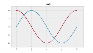
          plt.way.available # ['seaborn-dark', 'seaborn-darkgrid', 'seaborn-ticks', 'fivethirtyeight', #  'seaborn-whitegrid', 'archetype', '_classic_test', 'fast', 'seaborn-talk', #  'seaborn-dark-palette', 'seaborn-bright', 'seaborn-pastel', 'grayscale', #  'seaborn-notebook', 'ggplot', 'seaborn-colorblind', 'seaborn-muted', #  'seaborn', 'Solarize_Light2', 'seaborn-paper', 'bmh', 'tableau-colorblind10', #  'seaborn-white', 'dark_background', 'seaborn-poster', 'seaborn-deep']                  

          import matplotlib as mpl mpl.rcParams.update({'font.size': 18, 'font.family': 'STIXGeneral', 'mathtext.fontset': 'stix'})  def plot_sine_cosine_wave(style='ggplot'):     plt.style.use(style)     plt.effigy(figsize=(7,4), dpi=80)     X = np.linspace(0,2*np.pi,1000)     plt.plot(X,np.sin(X)); plt.plot(Ten,np.cos(10))     plt.xticks(ticks=np.arange(0, 440/57.2985, 90/57.2985), labels = [r'$0$',r'$\frac{\pi}{2}$',r'$\pi$',r'$\frac{iii\pi}{2}$',r'$2\pi$'])  # i radian = 57.2985 degrees     plt.gca().set(ylim=(-1.25, ane.25), xlim=(-.5, 7))     plt.title(fashion, fontsize=18)     plt.show()  plot_sine_cosine_wave('seaborn-notebook')     plot_sine_cosine_wave('ggplot')     plot_sine_cosine_wave('bmh')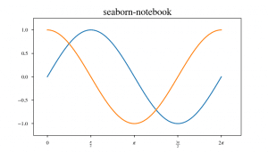                  

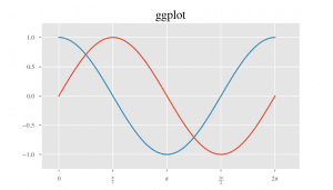
I've just shown few of the pre-built styles, the rest of the listing is definitely worth a wait.

Matplotlib too comes with pre-built colors and palettes. Type the post-obit in your jupyter/python panel to cheque out the available colors.

          # View Colors mpl.colors.CSS4_COLORS  # 148 colors mpl.colors.XKCD_COLORS  # 949 colors mpl.colors.BASE_COLORS  # viii colors #> {'b': (0, 0, 1), #>  'yard': (0, 0.5, 0), #>  'r': (1, 0, 0), #>  'c': (0, 0.75, 0.75), #>  'g': (0.75, 0, 0.75), #>  'y': (0.75, 0.75, 0), #>  'k': (0, 0, 0), #>  'w': (1, 1, i)}                  

          # View first x Palettes dir(plt.cm)[:10] #> ['Emphasis', 'Accent_r', 'Dejection', 'Blues_r', #>  'BrBG', 'BrBG_r', 'BuGn', 'BuGn_r', 'BuPu', 'BuPu_r']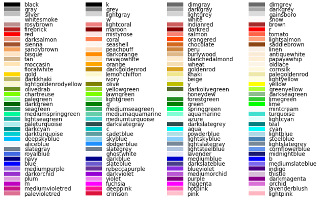                  

8. How to Customise the Legend

The most common way to make a legend is to define the label parameter for each of the plots and finally call plt.legend().

Notwithstanding, sometimes y'all might want to construct the legend on your own. In that case, yous need to pass the plot items you want to describe the legend for and the legend text as parameters to plt.legend() in the following format:

plt.legend((line1, line2, line3), ('label1', 'label2', 'label3'))

          # plt.style.employ('seaborn-notebook') plt.figure(figsize=(x,seven), dpi=lxxx) X = np.linspace(0, 2*np.pi, grand) sine = plt.plot(X,np.sin(X)); cosine = plt.plot(X,np.cos(10)) sine_2 = plt.plot(X,np.sin(Ten+.5)); cosine_2 = plt.plot(X,np.cos(10+.5)) plt.gca().set(ylim=(-1.25, 1.5), xlim=(-.v, seven)) plt.championship('Custom Legend Example', fontsize=18)  # Modify legend plt.legend([sine[0], cosine[0], sine_2[0], cosine_2[0]],   # plot items            ['sine curve', 'cosine curve', 'sine curve two', 'cosine curve 2'],              frameon=True,                                   # legend border            framealpha=1,                                   # transparency of border            ncol=2,                                         # num columns            shadow=True,                                    # shadow on            borderpad=ane,                                    # thickness of border            title='Sines and Cosines')                      # title plt.show()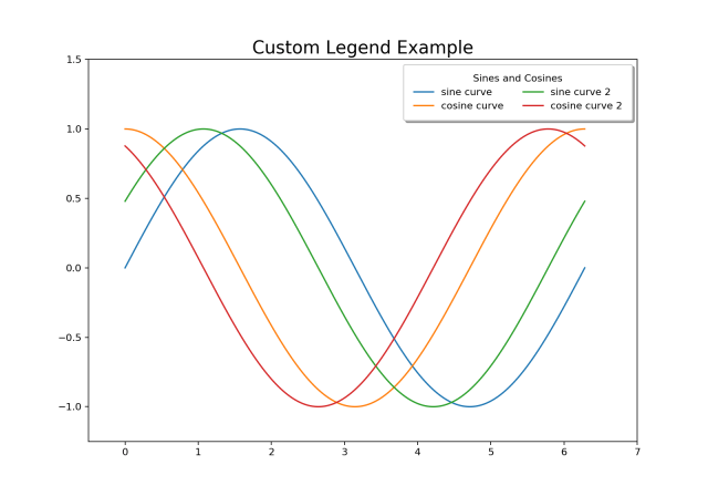                  

nine. How to Add Texts, Arrows and Annotations

plt.text and plt.annotate adds the texts and annotations respectively. If you take to plot multiple texts you need to telephone call plt.text() equally many times typically in a for-loop.

Let'due south comment the peaks and troughs adding arrowprops and a bbox for the text.

          # Texts, Arrows and Annotations Example # ref: https://matplotlib.org/users/annotations_guide.html plt.figure(figsize=(fourteen,7), dpi=120) X = np.linspace(0, viii*np.pi, g) sine = plt.plot(X,np.sin(X), color='tab:blue');  # ane. Annotate with Arrow Props and bbox plt.annotate('Peaks', xy=(90/57.2985, 1.0), xytext=(90/57.2985, 1.5),              bbox=dict(boxstyle='square', fc='green', linewidth=0.one),              arrowprops=dict(facecolor='greenish', shrink=0.01, width=0.1),               fontsize=12, color='white', horizontalalignment='eye')  # 2. Texts at Peaks and Troughs for angle in [440, 810, 1170]:     plt.text(angle/57.2985, 1.05, str(angle) + "\ndegrees", transform=plt.gca().transData, horizontalalignment='center', color='green')  for angle in [270, 630, 990, 1350]:     plt.text(angle/57.2985, -one.3, str(bending) + "\ndegrees", transform=plt.gca().transData, horizontalalignment='centre', colour='red')      plt.gca().gear up(ylim=(-2.0, two.0), xlim=(-.5, 26)) plt.title('Annotations and Texts Example', fontsize=18) plt.bear witness()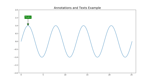                  

Notice, all the text we plotted higher up was in relation to the information.

That is, the x and y position in the plt.text() corresponds to the values along the ten and y axes. Notwithstanding, sometimes you lot might work with information of different scales on dissimilar subplots and you want to write the texts in the same position on all the subplots.

In such example, instead of manually calculating the x and y positions for each axes, y'all can specify the x and y values in relation to the axes (instead of 10 and y axis values).

You can practise this by setting transform=ax.transData.

The lower left corner of the axes has (x,y) = (0,0) and the superlative right corner volition represent to (1,1).

The below plot shows the position of texts for the same values of (x,y) = (0.50, 0.02) with respect to the Information(transData), Axes(transAxes) and Effigy(transFigure) respectively.

          # Texts, Arrows and Annotations Example plt.effigy(figsize=(14,7), dpi=80) X = np.linspace(0, 8*np.pi, 1000)  # Text Relative to Data plt.text(0.l, 0.02, "Text relative to the Information centered at : (0.50, 0.02)", transform=plt.gca().transData, fontsize=14, ha='heart', color='blue')  # Text Relative to AXES plt.text(0.fifty, 0.02, "Text relative to the AXES centered at : (0.l, 0.02)", transform=plt.gca().transAxes, fontsize=14, ha='eye', color='blueish')  # Text Relative to Figure plt.text(0.50, 0.02, "Text relative to the FIGURE centered at : (0.l, 0.02)", transform=plt.gcf().transFigure, fontsize=14, ha='center', colour='blue')  plt.gca().fix(ylim=(-2.0, ii.0), xlim=(0, ii)) plt.championship('Placing Texts Relative to Information, Axes and Figure', fontsize=eighteen) plt.show()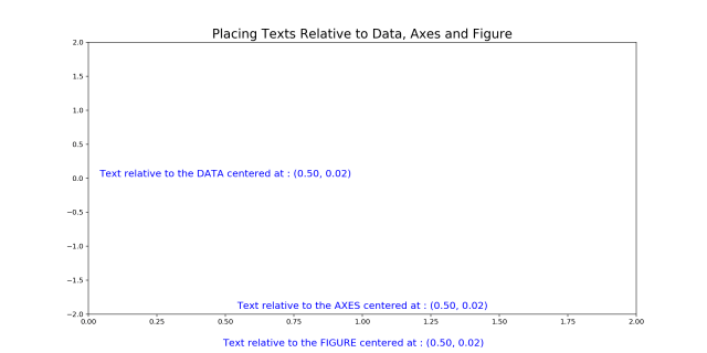                  

10. How to customize matplotlib'south subplots layout

Matplotlib provides ii convenient ways to create customized multi-subplots layout.

• plt.subplot2grid
• plt.GridSpec

Both plt.subplot2grid and plt.GridSpec lets you lot draw complex layouts. Below is a overnice plt.subplot2grid example.

          # Supplot2grid approach fig = plt.figure() ax1 = plt.subplot2grid((iii,iii), (0,0), colspan=2, rowspan=two) # topleft ax3 = plt.subplot2grid((3,3), (0,ii), rowspan=3)            # right ax4 = plt.subplot2grid((iii,3), (2,0))                       # bottom left ax5 = plt.subplot2grid((3,3), (2,1))                       # lesser right fig.tight_layout()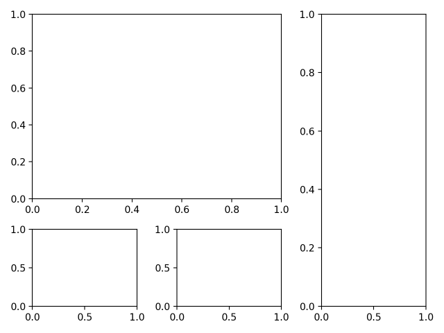                  

Using plt.GridSpec, you can use either a plt.subplot() interface which takes part of the filigree specified by plt.GridSpec(nrow, ncol) or employ the ax = fig.add_subplot(yard) where the GridSpec is divers past height_ratios and weight_ratios.

          # GridSpec Approach ane import matplotlib.gridspec as gridspec fig = plt.figure() grid = plt.GridSpec(2, three)  # 2 rows three cols plt.subplot(grid[0, :2])  # height left plt.subplot(grid[0, two])   # top right plt.subplot(grid[1, :ane])  # bottom left plt.subplot(grid[1, 1:])  # bottom correct fig.tight_layout()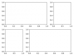                  

          # GridSpec Approach two import matplotlib.gridspec as gridspec fig = plt.figure() gs = gridspec.GridSpec(two, 2, height_ratios=[2,one], width_ratios=[1,2]) for m in gs:     ax = fig.add_subplot(thousand)     fig.tight_layout()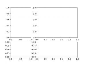                  

The above examples showed layouts where the subplots dont overlap. It is possible to make subplots to overlap. Infact y'all tin draw an axes inside a larger axes using fig.add_axes(). You demand to specify the ten,y positions relative to the figure and also the width and acme of the inner plot.

Beneath is an case of an inner plot that zooms in to a larger plot.

          # Plot inside a plot plt.way.use('seaborn-whitegrid') fig, ax = plt.subplots(figsize=(10,six)) x = np.linspace(-0.l, 1., one thousand)  # Outer Plot ax.plot(ten, x**2) ax.plot(ten, np.sin(x)) ax.set(xlim=(-0.5, one.0), ylim=(-0.5,ane.2)) fig.tight_layout()  # Inner Plot inner_ax = fig.add_axes([0.2, 0.55, 0.35, 0.35]) # 10, y, width, peak inner_ax.plot(10, x**two) inner_ax.plot(x, np.sin(x)) inner_ax.prepare(title='Zoom In', xlim=(-.2, .2), ylim=(-.01, .02),               yticks = [-0.01, 0, 0.01, 0.02], xticks=[-0.1,0,.1]) ax.set_title("Plot within a Plot", fontsize=20) plt.show() mpl.rcParams.update(mpl.rcParamsDefault)  # reset to defaults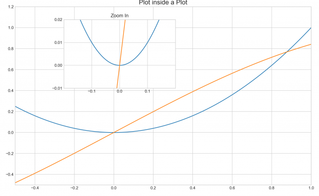                  

eleven. How is scatterplot drawn with plt.plot dissimilar from plt.scatter

The divergence is plt.plot() does non provide options to change the colour and size of indicate dynamically (based on some other array). Merely plt.scatter() allows you to do that.

By varying the size and colour of points, you can create overnice looking bubble plots.

Another convenience is you can directly use a pandas dataframe to prepare the x and y values, provided you lot specify the source dataframe in the data statement.

You tin too set the colour 'c' and size 'southward' of the points from one of the dataframe columns itself.

          # Scatterplot with varying size and color of points import pandas as pd midwest = pd.read_csv("https://raw.githubusercontent.com/selva86/datasets/master/midwest_filter.csv")  # Plot fig = plt.figure(figsize=(xiv, 7), dpi= lxxx, facecolor='westward', edgecolor='k')     plt.scatter('area', 'poptotal', data=midwest, s='dot_size', c='popdensity', cmap='Reds', edgecolors='black', linewidths=.v) plt.title("Bubble Plot of PopTotal vs Area\northward(color: 'popdensity' & size: 'dot_size' - both are numeric columns in midwest)", fontsize=16) plt.xlabel('Area', fontsize=18) plt.ylabel('Poptotal', fontsize=18) plt.colorbar() plt.evidence()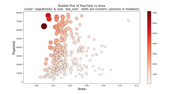                  

          # Import data import pandas as pd midwest = pd.read_csv("https://raw.githubusercontent.com/selva86/datasets/master/midwest_filter.csv")  # Plot fig = plt.effigy(figsize=(14, 9), dpi= fourscore, facecolor='westward', edgecolor='1000')     colors = plt.cm.tab20.colors categories = np.unique(midwest['category']) for i, category in enumerate(categories):     plt.besprinkle('area', 'poptotal', information=midwest.loc[midwest.category==category, :], due south='dot_size', c=colors[i], label=str(category), edgecolors='black', linewidths=.5)  # Legend for size of points for dot_size in [100, 300, thou]:     plt.scatter([], [], c='one thousand', alpha=0.5, s=dot_size, label=str(dot_size) + ' TotalPop') plt.fable(loc='upper right', scatterpoints=1, frameon=False, labelspacing=2, title='Saravana Stores', fontsize=8) plt.title("Bubble Plot of PopTotal vs Area\north(color: 'category' - a categorical column in midwest)", fontsize=18) plt.xlabel('Expanse', fontsize=16) plt.ylabel('Poptotal', fontsize=16) plt.show()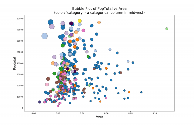                  

          # Save the figure plt.savefig("bubbleplot.png", transparent=Truthful, dpi=120)                  

12. How to depict Histograms, Boxplots and Fourth dimension Series

The methods to draw unlike types of plots are nowadays in pyplot (plt) as well as Axes. The beneath example shows basic examples of few of the commonly used plot types.

          import pandas as pd  # Setup the subplot2grid Layout fig = plt.figure(figsize=(10, 5)) ax1 = plt.subplot2grid((2,4), (0,0))  ax2 = plt.subplot2grid((two,iv), (0,i))  ax3 = plt.subplot2grid((ii,4), (0,2))  ax4 = plt.subplot2grid((2,4), (0,3))  ax5 = plt.subplot2grid((2,iv), (1,0), colspan=ii)  ax6 = plt.subplot2grid((2,4), (ane,2))  ax7 = plt.subplot2grid((ii,four), (1,3))   # Input Arrays n = np.array([0,1,2,3,4,5]) 10 = np.linspace(0,5,10) xx = np.linspace(-0.75, 1., 100)  # Scatterplot ax1.scatter(20, xx + np.random.randn(len(20))) ax1.set_title("Scatter Plot")  # Footstep Chart ax2.step(n, n**2, lw=2) ax2.set_title("Pace Plot")  # Bar Chart ax3.bar(n, n**2, align="center", width=0.5, alpha=0.5) ax3.set_title("Bar Chart")  # Fill up Between ax4.fill_between(10, x**2, 10**3, color="steelblue", blastoff=0.5); ax4.set_title("Fill Between");  # Time Series dates = pd.date_range('2018-01-01', periods = len(twenty)) ax5.plot(dates, xx + np.random.randn(len(xx))) ax5.set_xticks(dates[::xxx]) ax5.set_xticklabels(dates.strftime('%Y-%m-%d')[::30]) ax5.set_title("Fourth dimension Series")  # Box Plot ax6.boxplot(np.random.randn(len(xx))) ax6.set_title("Box Plot")  # Histogram ax7.hist(xx + np.random.randn(len(xx))) ax7.set_title("Histogram")  fig.tight_layout()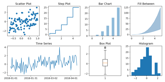                  

What about more advanced plots?

If you lot want to run across more information assay oriented examples of a particular plot blazon, say histogram or time series, the meridian 50 master plots for data analysis will give yous concrete examples of presentation ready plots. This is a very useful tool to take, not but to construct nice looking plots but to draw ideas to what type of plot y'all want to make for your data.

13. How to Plot with two Y-Axis

Plotting a line nautical chart on the left-hand side centrality is straightforward, which you lot've already seen.

So how to draw the second line on the correct-hand side y-axis?

The trick is to actuate the right hand side Y axis using ax.twinx() to create a second axes.

This second axes volition have the Y-axis on the right activated and shares the same x-centrality every bit the original ax. Then, whatever y'all draw using this 2nd axes volition exist referenced to the secondary y-axis. The remaining chore is to simply color the axis and tick labels to friction match the color of the lines.

          # Import Information df = pd.read_csv("https://github.com/selva86/datasets/raw/primary/economics.csv") 10 = df['appointment']; y1 = df['psavert']; y2 = df['unemploy']  # Plot Line1 (Left Y Axis) fig, ax1 = plt.subplots(1,1,figsize=(xvi,7), dpi= lxxx) ax1.plot(10, y1, color='tab:red')  # Plot Line2 (Right Y Axis) ax2 = ax1.twinx()  # instantiate a second axes that shares the same x-axis ax2.plot(x, y2, color='tab:bluish')  # Only Decorations!! ------------------- # ax1 (left y axis) ax1.set_xlabel('Twelvemonth', fontsize=xx) ax1.set_ylabel('Personal Savings Charge per unit', color='tab:ruddy', fontsize=20) ax1.tick_params(axis='y', rotation=0, labelcolor='tab:red' )  # ax2 (right Y centrality) ax2.set_ylabel("# Unemployed (chiliad's)", colour='tab:blue', fontsize=20) ax2.tick_params(axis='y', labelcolor='tab:blueish') ax2.set_title("Personal Savings Rate vs Unemployed: Plotting in Secondary Y Axis", fontsize=20) ax2.set_xticks(np.arange(0, len(x), 60)) ax2.set_xticklabels(x[::threescore], rotation=xc, fontdict={'fontsize':ten}) plt.prove()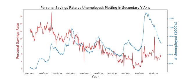                  

fourteen. Introduction to Seaborn

Every bit the charts get more complex, the more the code you've got to write. For case, in matplotlib, there is no direct method to draw a density plot of a scatterplot with line of best fit. Yous get the thought.

And so, what you can practise instead is to use a higher level packet similar seaborn, and utilize 1 of its prebuilt functions to draw the plot.

We are not going in-depth into seaborn. Merely let's see how to get started and where to detect what you lot desire. A lot of seaborn's plots are suitable for data analysis and the library works seamlessly with pandas dataframes.

seaborn is typically imported equally sns. Like matplotlib it comes with its own gear up of pre-built styles and palettes.

          import seaborn as sns sns.set_style("white")  # Import Information df = pd.read_csv("https://github.com/selva86/datasets/raw/chief/mpg_ggplot2.csv")  # Describe Plot plt.figure(figsize=(sixteen,ten), dpi= 80) sns.kdeplot(df.loc[df['cyl'] == iv, "cty"], shade=True, color="g", label="Cyl=4", alpha=.7) sns.kdeplot(df.loc[df['cyl'] == 6, "cty"], shade=True, color="dodgerblue", label="Cyl=6", alpha=.7) sns.kdeplot(df.loc[df['cyl'] == viii, "cty"], shade=True, color="orange", characterization="Cyl=viii", alpha=.7)  # Ornamentation plt.title('Density Plot of City Mileage by n_Cylinders', fontsize=22) plt.fable() plt.show()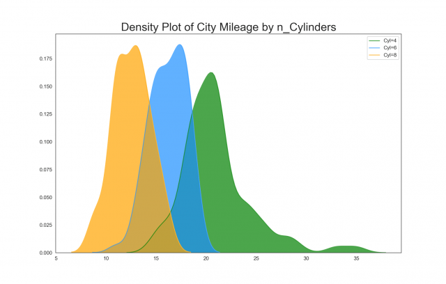                  

          # Load Dataset df = sns.load_dataset('iris')  # Plot plt.figure(figsize=(10,8), dpi= 80) sns.pairplot(df, kind="reg", hue="species") plt.show()                  

          <Figure size 800x640 with 0 Axes>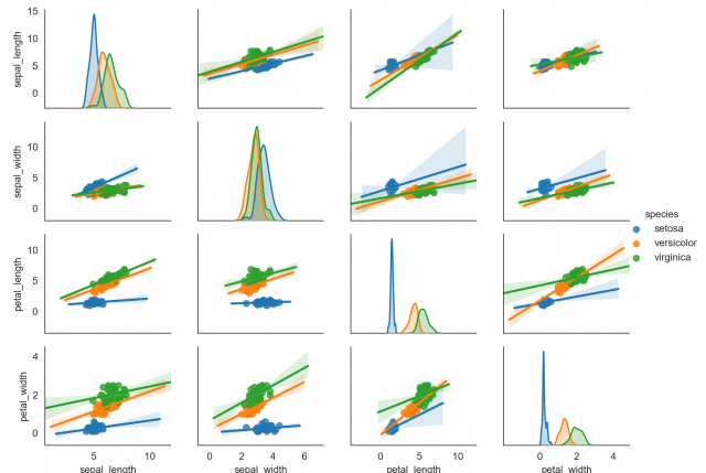                  

This is just to give a hint of what's possible with seaborn. Perchance I will write a separate mail service on it. However, the official seaborn folio has practiced examples for you lot to start with.

xv. Determination

Congratulations if you reached this far. Because we literally started from scratch and covered the essential topics to making matplotlib plots.

We covered the syntax and overall structure of creating matplotlib plots, saw how to modify various components of a plot, customized subplots layout, plots styling, colors, palettes, depict different plot types etc.

If you lot want to get more practice, endeavour taking upward couple of plots listed in the top 50 plots starting with correlation plots and endeavour recreating it.

Until next time

Source: https://www.machinelearningplus.com/plots/matplotlib-tutorial-complete-guide-python-plot-examples/

Posted by: howellproself.blogspot.com

Share this post